How to highlight duplicates in Excel

While working with huge datasets in Excel, you may need to find and eliminate duplicate values. Applying different styles to cells based on whether or not they meet specific conditions is possible with conditional formatting.
This tutorial will demonstrate how to highlight duplicates in Excel.
How to highlight duplicates in Excel
Here are the steps on how to highlight duplicates in Excel:
- Choose the data that you suspect may be duplicated.
- Click Home > Conditional Formatting > Highlight Cells Rules > Duplicate Values.
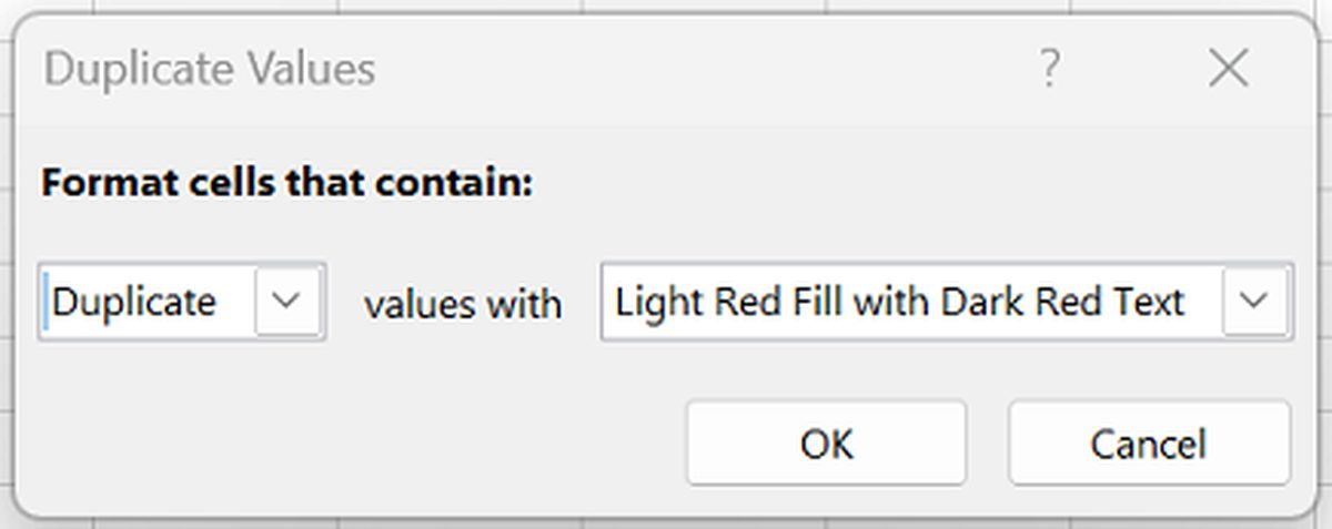
- By default, when you open the Duplicate Values dialogue box, the Fill color will be Light Red, and the Text color will be Dark Red. Choose OK to use the predefined setting.
- To change the format, go to Format and choose a new one from the drop-down menu.
- To use the new layout, select OK.
The duplicates in the chosen range will now be highlighted.
To get rid of duplicates in your data, utilize the Remove Duplicates tool. Choose the records from which you wish to eliminate duplicates, and then go to Data > Remove Duplicates.
You can use conditional formatting to highlight other types of data, such as cells that contain errors or cells that are above or below a certain value.
Excel tips & tricks
If you use Excel frequently, you might be interested in some tips and tricks to make your work easier and more efficient, such as:
- Use keyboard shortcuts: Keyboard shortcuts can save you a lot of time and clicks when working with Excel. For example, you can use Ctrl+C to copy, Ctrl+V to paste, Ctrl+Z to undo, Ctrl+F to find, and so on. You can also use F2 to edit a cell, F4 to repeat the last action, F9 to recalculate all formulas, and F11 to create a chart from the selected data.

- Use formulas and functions: Formulas and functions are the core of Excel. They allow you to perform calculations, manipulate data, and analyze information. For example, you can use SUM to add up a range of numbers, AVERAGE to find the mean value, IF to test a condition, VLOOKUP to look up a value in a table, and so on. You can also combine formulas and functions to create more complex calculations.
- Use data validation: Data validation is a feature that allows you to control what kind of data can be entered in a cell or a range of cells. For example, you can use data validation to restrict the input to numbers only, dates only, a list of predefined options, or a custom rule. You can also use data validation to display an input message or an error message when someone enters invalid data.
- Use conditional formatting: Conditional formatting is a feature that allows you to apply different formats to cells or ranges of cells based on certain criteria. For example, you can use conditional formatting to highlight the highest or lowest values in a column, color-code the cells based on their values, or show icons or bars to indicate the performance of the data.
- Use pivot tables and charts: Pivot tables and charts are powerful tools that allow you to summarize, analyze, and visualize your data. You can use pivot tables and charts to create reports, dashboards, and interactive tables and graphs. You can also use pivot tables and charts to filter, sort, group, and drill down your data.
Advertisement